Original Research · Computational Re-Analysis
County-level determinants of cancer incidence in the United States, and the drivers of Iowa's rising rate
An unbiased, multi-method ecological re-analysis across approximately 3,100 counties and the 1999–2023 national incidence series.
1 Independent research, Iowa, USA. Correspondence: msnellered@gmail.com
Highlights
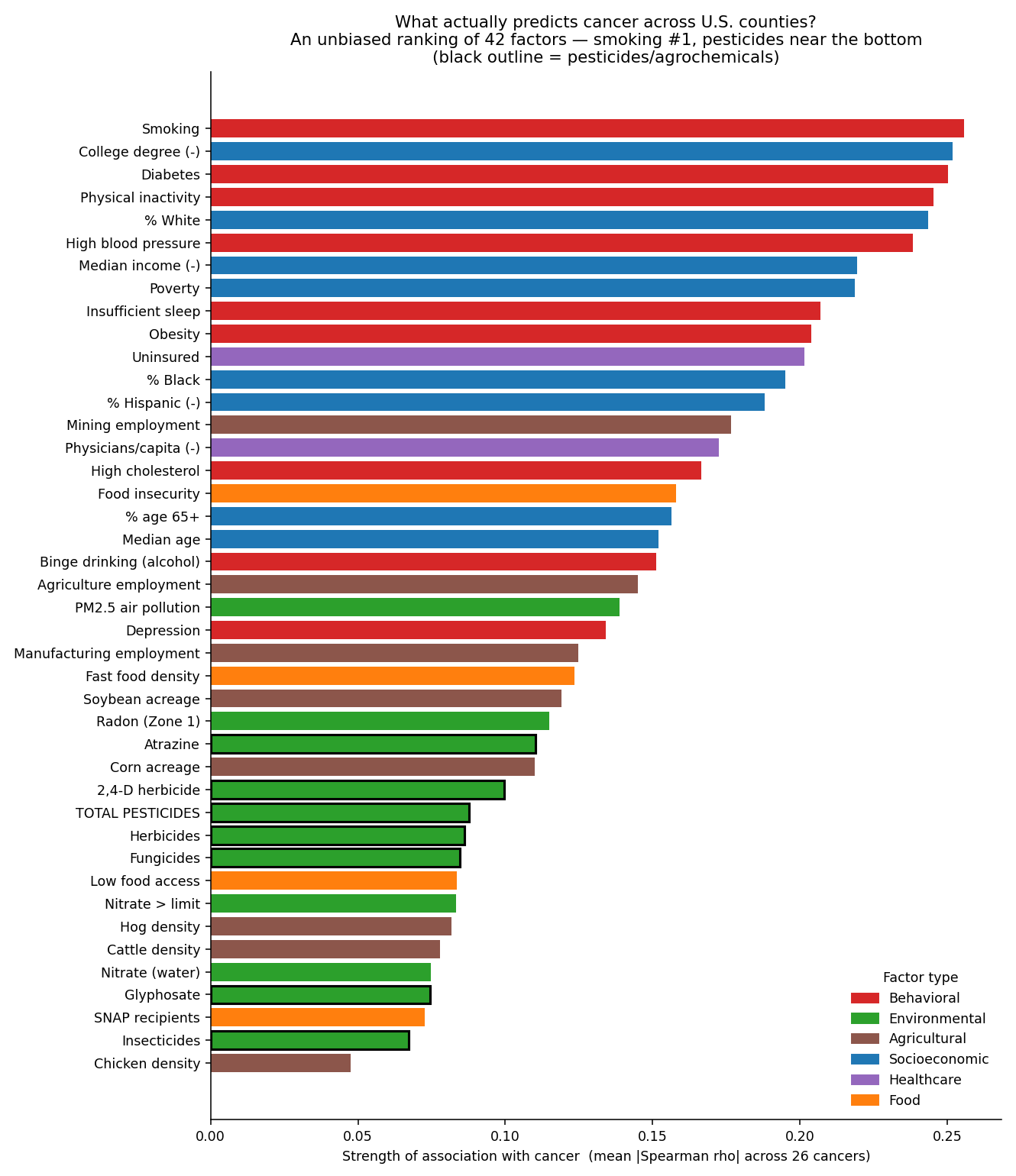
- Across 42 county-level factors scored against 26 cancer sites, smoking ranks first; agricultural pesticides rank 31st.
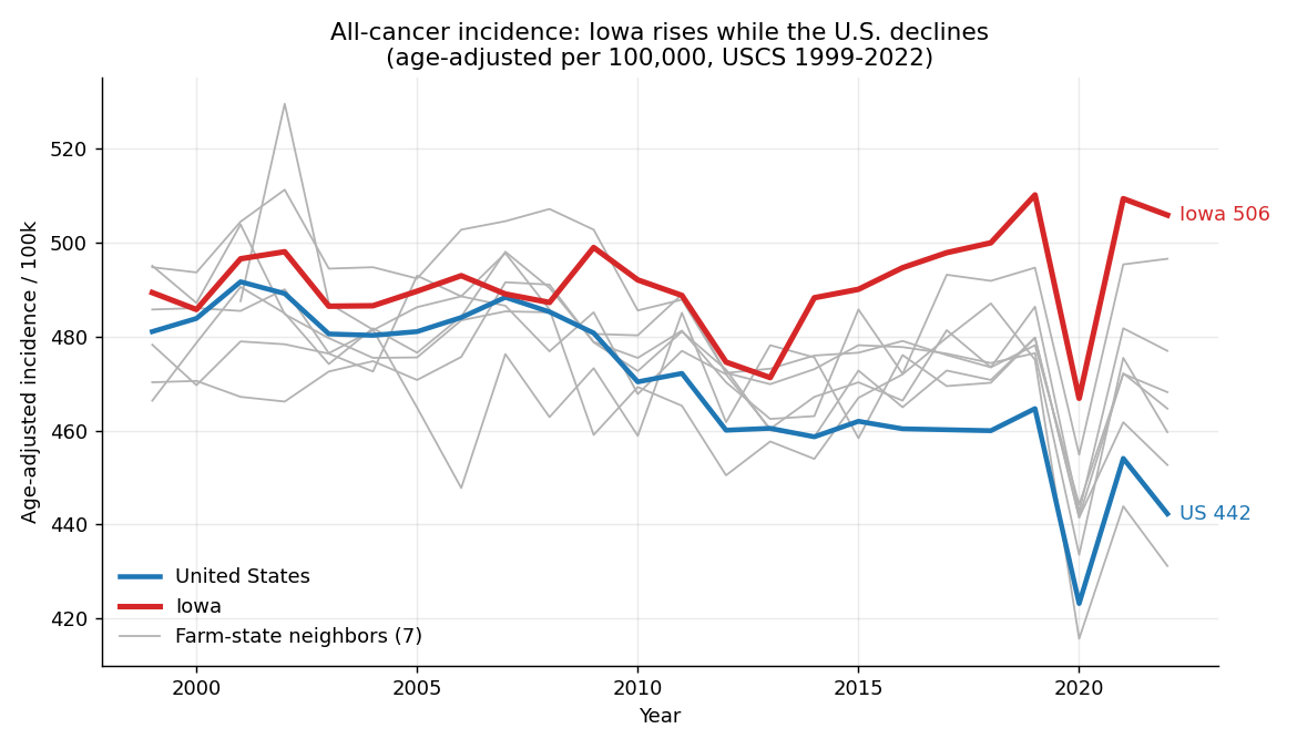
- Iowa's age-adjusted incidence stayed approximately flat (1999–2019) while the national rate declined by about 5 percent.
- The divergence reflects a stalled decline plus detection and overdiagnosis, alcohol, and ultraviolet exposure, not a new carcinogen.
- A farm-state natural experiment and within-Iowa null associations do not support pesticides as the driver.
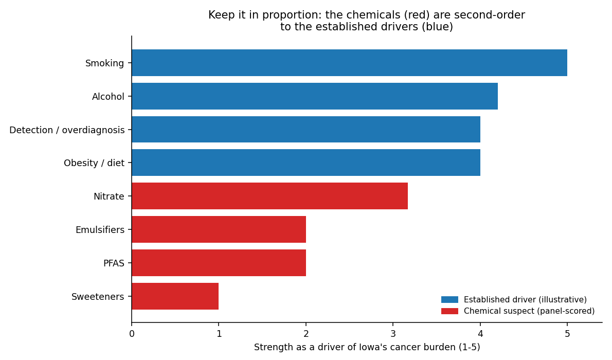
- Four candidate water and food chemicals rank as second-order; drinking-water nitrate is the most defensible for Iowa.
Abstract
Background. Ecological studies have linked agricultural chemicals to cancer, often within a single-hypothesis framework. Iowa is one of only a few U.S. states with a rising age-adjusted incidence rate, and the cause is unsettled.
Methods. We re-analysed county-level incidence for 26 cancer sites against 42 candidate exposures using rank correlation with Benjamini–Hochberg control, random-forest permutation importance, and LASSO. We reconstructed the 1999–2023 state series (U.S. Cancer Statistics) to decompose Iowa's trajectory by site and by incidence versus mortality, ranked all 50 states by trend, and assessed four candidate chemical exposures (drinking-water nitrate, PFAS, dietary emulsifiers, non-nutritive sweeteners) against current evidence with an independent three-rater scoring panel. All results regenerate from committed scripts.
Results. Smoking was the strongest county-level correlate; total pesticide density ranked 31 of 42 and did not survive calibration against established carcinogens (the smoking to lung association was approximately 11 times larger). Iowa's age-adjusted rate held roughly flat while the national rate fell, widening the gap from about +8 to between +45 and +64 per 100,000. Rising sites (kidney, thyroid, melanoma) showed incidence increasing faster than mortality, the signature of detection and overdiagnosis; the fastest-rising sites were ultraviolet and alcohol related. Among chemical hypotheses, nitrate was the most defensible (median Iowa exposure lies within the band where cohorts detect effects, below a limit set in 1962 for an infant condition rather than cancer), PFAS an established hazard at serum doses Iowans rarely reach, emulsifiers mechanistically plausible but null for colorectal cancer in cohort, and sweeteners the least supported.
Conclusions. Established behavioural and socioeconomic factors dominate U.S. county cancer variation. Iowa's rise is best explained by a stalled decline in smoking-related and screen-detected cancers together with a high alcohol and ultraviolet burden, not by a novel environmental carcinogen. Candidate chemical exposures are at most second-order and require individual-level designs to test. Findings are ecological and hypothesis-generating, not evidence of individual-level causation.
Keywords: ecological epidemiology; cancer incidence; age-adjusted trends; Iowa; nitrate; PFAS; gut microbiome; overdiagnosis; confounding; reproducibility.
Introduction
A prior version of this project, despite an extensive analytical apparatus, was structured to confirm a single hypothesis: that agricultural pesticides cause cancer. Its competing-risk analyses were framed to defend that signal rather than to weigh alternatives on equal terms, it did not examine Iowa, and a key environmental covariate (radon) was never obtained. This re-analysis reopens the two questions the prior framing could not answer without bias: which factors actually predict cancer across U.S. counties when none is privileged, and why Iowa's age-adjusted incidence is rising while most states decline.
We adopt three disciplines throughout. No exposure is favoured a priori; effect sizes are calibrated against established carcinogens; and association is kept distinct from causation, hazard from risk, and detection from true incidence. The honest answers below overturn the original conclusion, which is the point of an unbiased design.
What predicts cancer across counties
Forty-two candidate factors were scored against all 26 cancer sites on equal footing. Smoking is the strongest correlate in the dataset, within a tight cluster of socioeconomic and metabolic factors. Pesticides rank in the bottom third (31st of 42; glyphosate 39th), a placement robust to resampling. In a common regression the herbicide to kidney association is real but small (about +1.6 percent per standard deviation), whereas the smoking to lung association is approximately +17.6 percent, an order of magnitude larger.
Why Iowa is rising
Iowa's age-adjusted all-cancer incidence is approximately flat since 1999 (+0.06 percent per year), but the national rate fell by about 5 percent over the same period. Iowa therefore diverged upward by failing to decline. Decomposition attributes most of the gap to a slower fall in prostate and lung cancer (a smoking legacy sustained by weak tobacco-control policy), while the fastest-rising sites are ultraviolet related (melanoma) and alcohol related (liver, oral cavity, oesophagus). For kidney, thyroid, and melanoma, incidence rises far faster than mortality, the established signature of screening and incidental detection rather than rising lethality. A natural experiment reinforces the point: neighbouring farm states that apply the same pesticides declined like the nation, and within Iowa no single measured factor explains the county pattern.
Candidate chemical exposures
We assessed four chemicals proposed to act through the gut microbiome or as direct toxicants, scored by an independent three-rater panel for mechanistic plausibility, human evidence, dose realism at Iowa exposure, local relevance, and testability. None reaches a high score as a driver of Iowa's burden, and all sit below the established causes (smoking, alcohol, obesity, detection). Drinking-water nitrate is the most defensible: Iowa's median exposure lies within the range where prospective cohorts report effects, yet below a standard set in 1962 for an infant condition rather than cancer.
| Exposure | Medium | Overall | Status |
|---|---|---|---|
| Nitrate | Drinking water | 3.2 | Plausibly a minor cause; most Iowa-relevant |
| PFAS | Drinking water | 2.0 | Established hazard, but doses Iowans rarely reach |
| Emulsifiers | Ultra-processed food | 2.0 | Strong mechanism, null for colorectal in cohort |
| Sweeteners | Food and drink | 1.0 | Least supported; possibly net protective |
Limitations
This is an ecological design: county-level associations need not hold at the individual level (the ecological fallacy), and a known carcinogen, radon, even reverses sign against lung cancer here because high-radon rural counties smoke less. The age-stratified data are national, so Iowa's early-onset signal cannot be localised in this dataset. The chemical assessments draw on the published literature and, for nitrate and PFAS, real exposure data, but the ecological layer cannot establish causation. The work is hypothesis-generating; the decisive tests are individual-level, described in the linked sections.
Selected sources
- U.S. Cancer Statistics (USCS), CDC and NCI, incidence and mortality, 1999–2023.
- State Health Registry of Iowa. Cancer in Iowa, annual reports 2023–2026.
- IARC Monographs Vol. 135 (perfluorooctanoic acid, perfluorooctanesulfonic acid), 2025; aspartame evaluation (Group 2B), 2023.
- Schullehner J, et al. Nitrate in drinking water and colorectal cancer risk. Int J Cancer. 2018.
- Spaur M, et al. Drinking-water nitrate and prostate cancer in the Agricultural Health Study. J Natl Cancer Inst. 2026.
- Chassaing B, et al. Randomized controlled-feeding trial of carboxymethylcellulose. Gastroenterology. 2022.
- Suez J, et al. Personalized microbiome-driven effects of non-nutritive sweeteners. Cell. 2022.
- Díaz-Gay M, Alexandrov LB, et al. Geographic and age variation in colorectal-cancer mutational signatures. Nature. 2025.
- Shearer JJ, et al. Serum PFOA and renal cell carcinoma (PLCO). J Natl Cancer Inst. 2021.
- U.S. EPA. Fifth Unregulated Contaminant Monitoring Rule (UCMR5) occurrence data, 2023–2025.