Study Design Overview
This is a county-level ecological study. The unit of observation is the US county (n=3,248). The exposure is agricultural pesticide application density (kg/mi², 2019 USGS PNSP estimates). The outcomes are age-adjusted cancer incidence rates (per 100,000, 2016–2020 NCI State Cancer Profiles). We control for 9–13 confounders depending on model specification.
Confounders
- Demographics: median household income, poverty rate, % college degree, % 65+, median age
- Health behaviors: smoking prevalence, obesity prevalence, physical inactivity
- Additional (v2A): binge drinking, food insecurity, % low food access
- Agricultural (v2B): nitrate water contamination (mg/L)
1. Bivariate Correlations
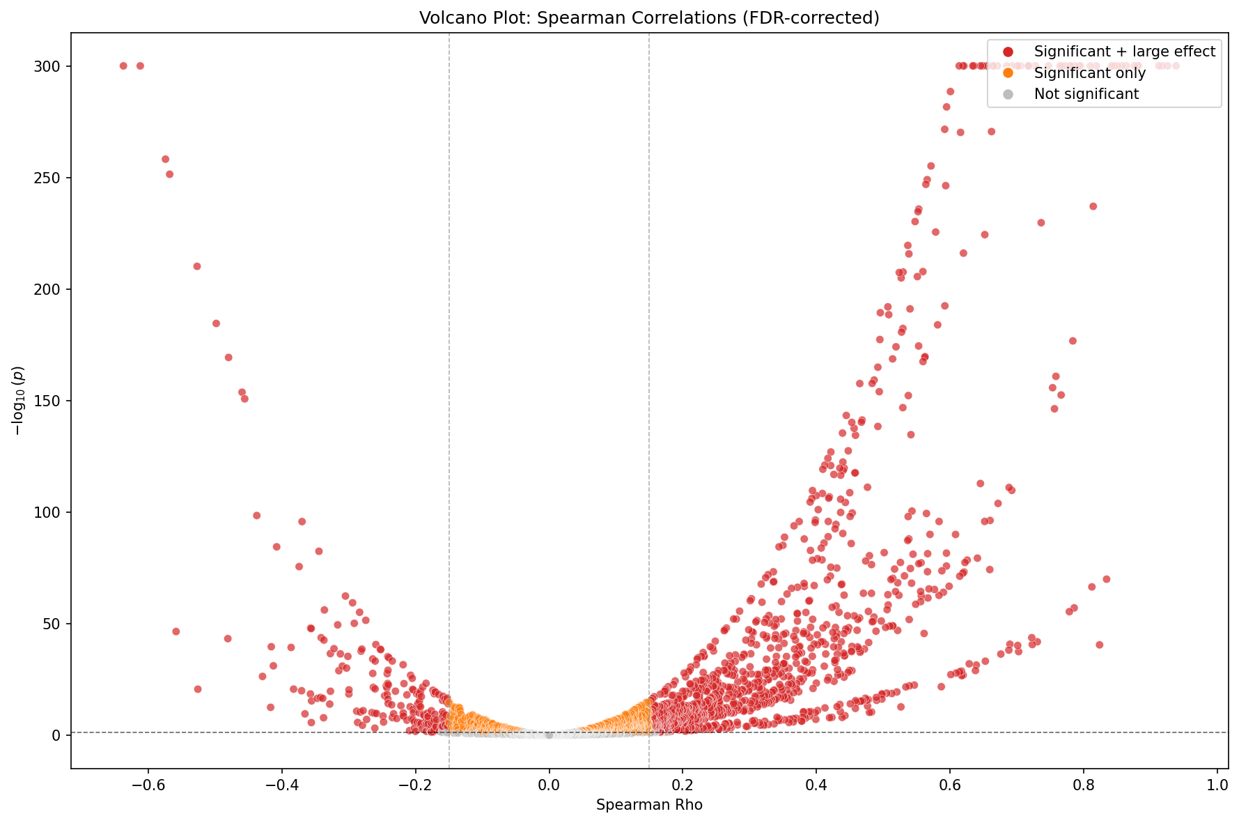
Spearman Rank Correlations
Non-parametric correlations between pesticide density and each cancer type. Does not control for confounders; establishes whether any crude association exists. Spearman is robust to non-normal distributions common in county-level health data.
Partial Correlations
Spearman correlations controlling for 9 confounders simultaneously. Tests whether the pesticide–cancer association survives basic confounding control.
2. Multivariate Regression
OLS Regression
Standard ordinary least squares with all confounders. Provides interpretable coefficients but assumes independent observations (violated by spatial autocorrelation).
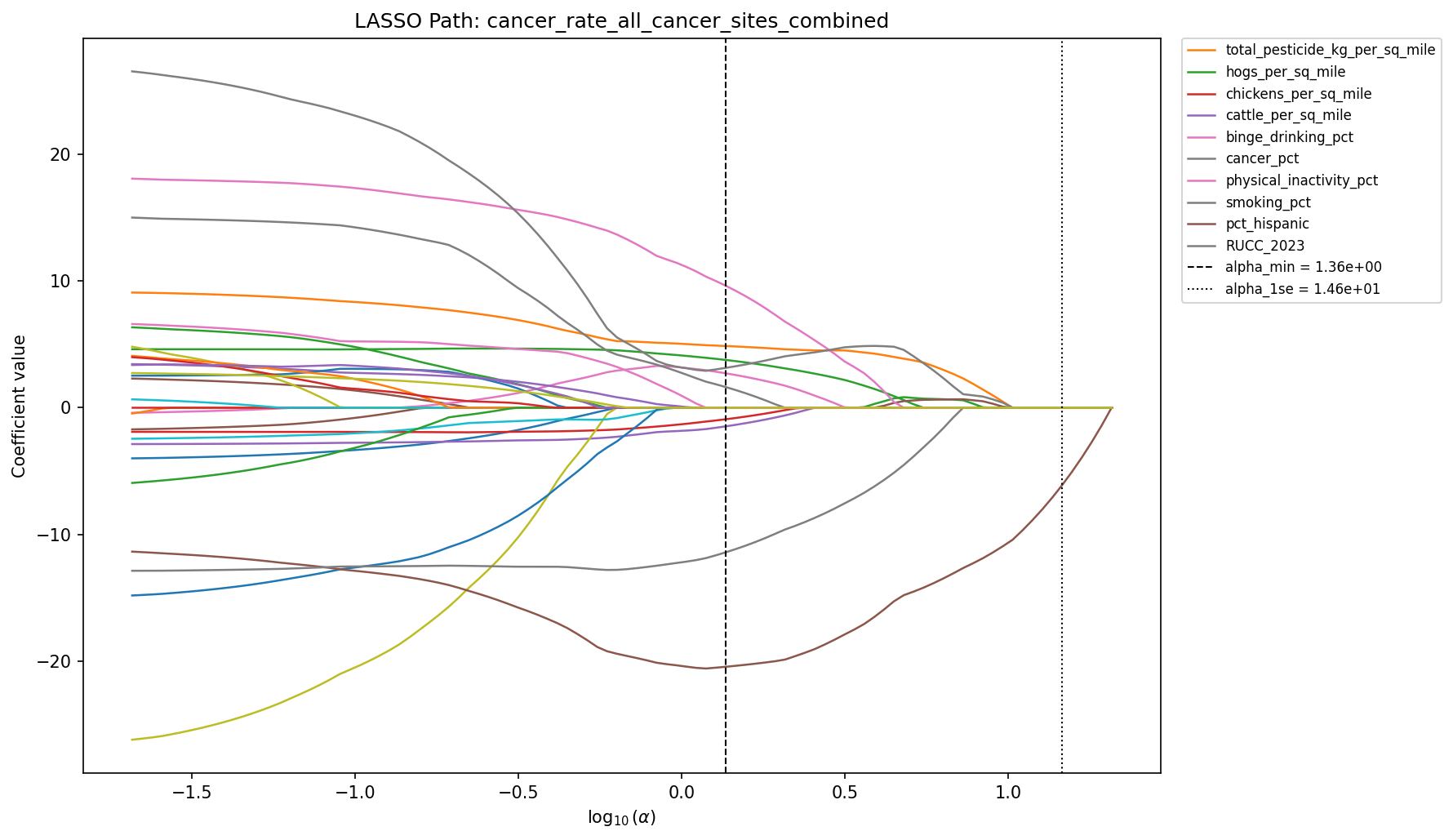
LASSO (L1 Regularization)
LASSO selects the most predictive variables from 29 candidates via cross-validation. Pesticide is retained among the top 10 selected variables, confirming it adds predictive value beyond the other confounders.
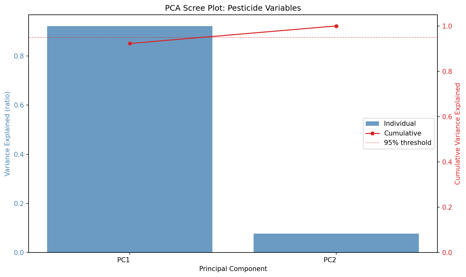
PCA + Regression
Principal Component Analysis on the pesticide variables (total, herbicide, insecticide, fungicide) to address multicollinearity among pesticide subtypes.
3. Spatial Regression
Moran’s I & LISA
Global Moran’s I confirms significant spatial autocorrelation in cancer rates (I > 0.3 for most types). LISA (Local Indicators of Spatial Association) identifies hot/cold spot clusters. This motivates the use of spatial regression models.
Spatial Error & Spatial Lag Models
Spatial Error models account for spatially correlated residuals (unobserved spatially varying confounders). Spatial Lag models account for spillover effects between neighboring counties. Spatial Error wins for 43 of 44 cancer-type tests by AIC.
Geographically Weighted Regression (GWR)
GWR allows coefficients to vary locally, revealing spatial heterogeneity in the pesticide effect. Bandwidth = 133 counties; mean R² = 0.495. About 9% of counties show significant positive pesticide effects, 7.5% significant negative, and 83.4% non-significant.
Spatial Durbin Model
Incorporates both spatially lagged dependent variable and spatially lagged covariates. Wins by AIC (21,312) over Spatial Error (29,246) and Spatial Lag (29,309), indicating that both neighbor effects and spillovers matter.
4. Causal Identification
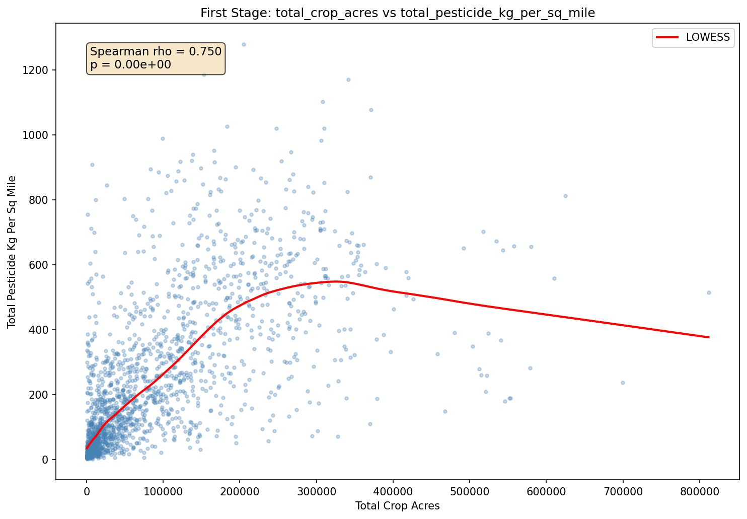
Instrumental Variables (IV/2SLS)
Uses total crop acreage as an instrument for pesticide application. Crop acreage predicts pesticide use (first-stage F=377.8) but should not directly cause cancer except through pesticide exposure. The IV estimate (0.035) exceeds OLS (0.019), suggesting attenuation bias from measurement error rather than confounding bias.
Long-Difference Estimator
Computes Δpesticide (2012 minus 1997) and Δcancer rate for each county. By examining within-county changes over 15 years, this eliminates all time-invariant confounders. Controls for 11 baseline covariates. Kidney (β=0.068, p=0.003) and colorectal (β=0.079, p<0.001) are significant; all-site and NHL are null.
5. Bayesian Spatial Models (BYM2)
The BYM2 (Besag-York-Mollié 2) model is the gold standard for disease mapping. It decomposes county-level variation into:
- Fixed effects: pesticide exposure + 9–13 confounders
- Spatially structured random effects: ICAR (intrinsic conditional autoregressive) component capturing smooth spatial trends
- Unstructured random effects: county-specific noise
- ρ (rho): mixing parameter between structured and unstructured components
High ρ values (0.93–0.99) indicate most residual variation is spatially structured, meaning the spatial random effects absorb substantial unmeasured spatial confounding. The fact that pesticide effects survive this aggressive spatial smoothing is notable.
Model Specifications
v1 (9 covariates): demographics + health behaviors + SES.
v2A (12 covariates): + binge drinking, food insecurity, food access.
v2B (13 covariates): + nitrate water contamination (key agricultural confounder test).
All models: 3,000 tuning + 1,500 draw iterations, nutpie sampler, Poisson likelihood with expected-count offset.
6. Compound & Pathway Analysis
Compound-Specific BYM2
12 individual compounds tested in separate BYM2 models (each with 12 baseline covariates). Six herbicides, three insecticides, three fungicides. Tests whether the signal is driven by specific chemical classes or is a generic agricultural-intensity artifact.
Exposure Pathway Stratification
BYM2 models run separately on urban (RUCC 1–3) and rural (RUCC 4–9) county subsets. If the association were purely occupational, we would expect it only in rural counties. Similar RRs in both strata suggest dietary or ubiquitous environmental exposure.
7. Positive Control Validation
The PM2.5–lung cancer relationship is well-established (meta-analytic RR ≈ 1.10–1.15 per 10 μg/m³). We tested this in our pipeline: the IV/2SLS estimate yields a 17.9% relative increase per 10 μg/m³, consistent with published estimates. This confirms the pipeline can detect known environmental carcinogens.
Methods Comparison
| Analysis | Pesticide Effect | Spatial Control | Interpretation |
|---|---|---|---|
| Spearman Correlation | Positive, significant | None | Crude association exists |
| Partial Correlation | Positive, significant | Confounders only | Survives basic confounding |
| OLS Regression | Positive, significant | None | Multivariate effect is small but real |
| LASSO Selection | Selected (10/29 vars) | Regularization | Adds predictive value |
| Spatial Error Model | Attenuated | Spatial autocorrelation | Wins for 43/44 cancer types |
| GWR | 9% sig+, 7.5% sig− | Locally varying | Spatially heterogeneous |
| Spatial Durbin | Lowest AIC model | Spillovers + lag | Neighbor effects matter |
| IV / 2SLS | IV > OLS (0.035 vs 0.019) | Endogeneity (F=377.8) | OLS biased toward zero |
| Long-Diff Kidney | β=0.068, p=0.003 | Within-county Δ | Temporal variation confirms signal |
| Long-Diff Colorectal | β=0.079, p<0.001 | Within-county Δ | Temporal variation confirms signal |
| BYM2 v1 All-Site | Null (RR ≈ 1.00) | Full BYM2 (ρ=0.997) | Spatial RE absorbs all-site signal |
| BYM2 v1 Kidney | RR=1.025, P(>0)=0.997 | Full BYM2 (ρ=0.986) | SURVIVES spatial smoothing |
| BYM2 v1 Colorectal | RR=1.015, P(>0)=0.991 | Full BYM2 (ρ=0.989) | SURVIVES spatial smoothing |
| BYM2 v2B Kidney | RR=1.034, P(>0)=0.997 | + nitrate (ρ=0.971) | ROBUST to agricultural confounding |
| BYM2 v2B Colorectal | RR=1.018, P(>0)=0.991 | + nitrate (ρ=0.939) | ROBUST to agricultural confounding |
| Compound BYM2 | Herbicides sig, insecticides NS | Compound-level BYM2 | Chemical class specificity |
| Neg Controls | Livestock/diabetes NS | Alternative exposures | Not agricultural intensity |
| Pathway BYM2 | Urban RR ≈ Rural RR | Stratified BYM2 | Dietary/ubiquitous pathway |
| Smoking Gauntlet | Pest kidney survives | Covariate in BYM2 | Independent of smoking |
| Obesity Gauntlet | Both kidney covariates sig | Covariate in BYM2 | Independent risk pathways |
| Alcohol Gauntlet | Pest CRC survives (alcohol NS) | Covariate in BYM2 | Not alcohol confounding |
| Inactivity Gauntlet | Both pest covariates survive | Covariate in BYM2 | Independent of inactivity |
| Exploratory Screen | Pest top for kidney/CRC | 26 cancers × all predictors | Hypothesis-free confirmation |
8. Risk Factor Gauntlets
Each IARC-established carcinogen (smoking, obesity, alcohol, physical inactivity) is tested as a primary exposure across 12 cancer types using three methods: BYM2, long-difference, and IV/2SLS. The pesticide covariate is included in every gauntlet model to test whether it survives as a covariate.
- BYM2: Same spatial model as above, but with each risk factor as primary exposure + pesticide as covariate
- Long-difference: Uses County Health Rankings historical data (2010–2024) to compute within-county changes in risk factor prevalence
- IV/2SLS: Risk factor-specific instruments (e.g., convenience stores for smoking, food environment for obesity, RUCC for inactivity)
This design tests two things simultaneously: (1) whether each risk factor itself shows expected IARC-linked cancer patterns, and (2) whether pesticide associations are independent of that risk factor. See full results on the Gauntlets page.
9. Exploratory Screening
A hypothesis-free scan of all available predictors against all 26 cancer types. Four analytical layers:
- Spearman correlations with Benjamini-Hochberg FDR correction (q < 0.05)
- Partial correlations controlling for 9 baseline confounders
- LASSO variable selection via cross-validated regularization
- OLS regression with all predictors surviving LASSO selection
This complements hypothesis-driven analysis by asking: among all possible predictors, does pesticide emerge as a top correlate for the same cancer types identified by BYM2? See Exploratory page.
10. Temporal Cancer Panel
Cancer incidence panel data from CDC EPHT (9 cancer types, 16 rolling 5-year windows from 2001–2020, 2,727 counties). Animated choropleth maps show how geographic patterns evolve over time. Combined with pesticide application trends and health behavior trends from County Health Rankings. See Temporal Trends page.
11. Sensitivity Analyses
- Bootstrap confidence intervals: 1,000 resamples for correlation and regression estimates
- Leave-one-state-out: Jackknife across all 50 states; association remains positive in all iterations
- Suppressed-county sensitivity: Results stable under varying county-inclusion thresholds
- Lag window sensitivity: Tests different exposure-outcome temporal gaps
- Outlier robustness: Cook’s distance and IQR-based trimming; results unchanged