Surviving Associations
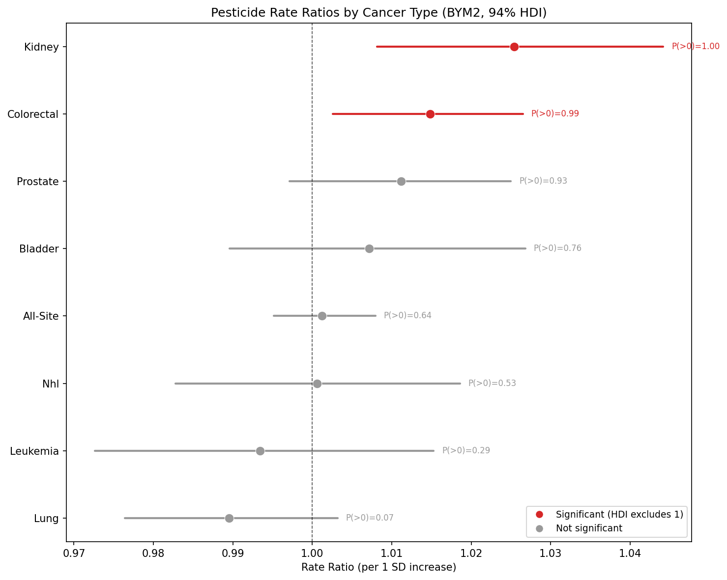
Of eight cancer types tested in BYM2 Bayesian spatial models, only kidney and colorectal cancer show statistically credible associations with total pesticide application that survive all model specifications.
Confounding Robustness
The pesticide–kidney and pesticide–colorectal associations were tested across five progressively inclusive model specifications. Rate ratios remain stable or strengthen as confounders are added.
| Model | Covariates Added | Kidney RR | P(>0) | ρ | Colorectal RR | P(>0) | ρ |
|---|---|---|---|---|---|---|---|
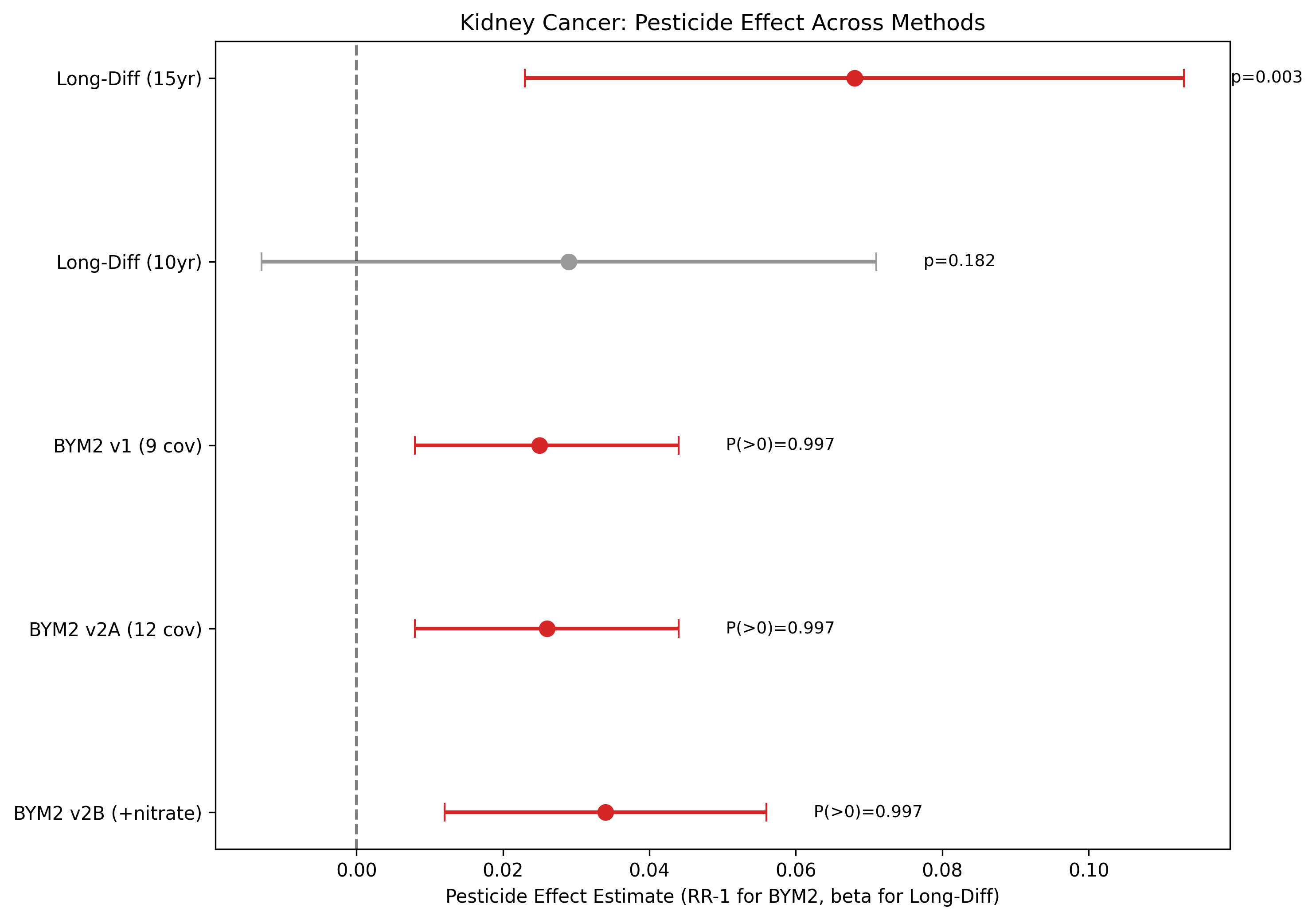
| BYM2 v1 (9 cov) | Baseline: demographics, health, SES | 1.025 | 0.997 | 0.986 | 1.015 | 0.991 | 0.989 |
| BYM2 v2A (12 cov) | + food insecurity, food access, binge drinking | 1.026 | 0.997 | 0.982 | 1.015 | 0.987 | 0.988 |
| BYM2 v2B (13 cov) | + nitrate water contamination | 1.034 | 0.997 | 0.971 | 1.018 | 0.991 | 0.939 |
| + Livestock (NB 15) | + hog/cattle/chicken density (all NS) | 1.025 | 0.997 | 0.986 | 1.015 | 0.991 | 0.989 |
| + Diabetes (NB 15) | + diabetes prevalence (NS) | 1.025 | 0.997 | 0.986 | 1.015 | 0.991 | 0.989 |
Key: Nitrate Does Not Confound
Adding nitrate water contamination (a plausible agricultural confounder) to BYM2 v2B actually strengthens the kidney RR from 1.025 to 1.034, while nitrate itself is null for all cancer types. This rules out the hypothesis that the pesticide signal is merely a proxy for agricultural water pollution.
Compound Specificity
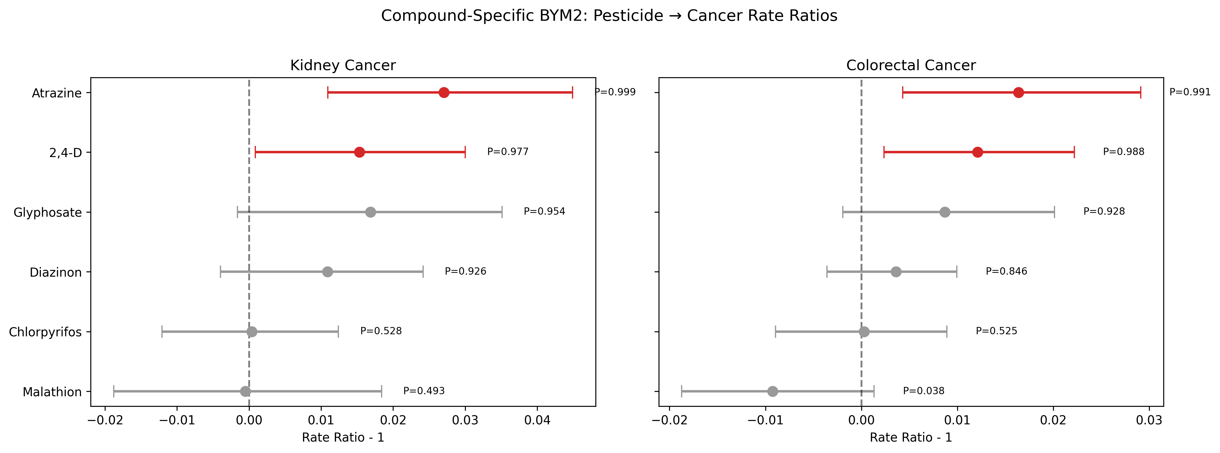
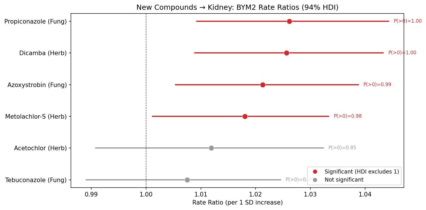
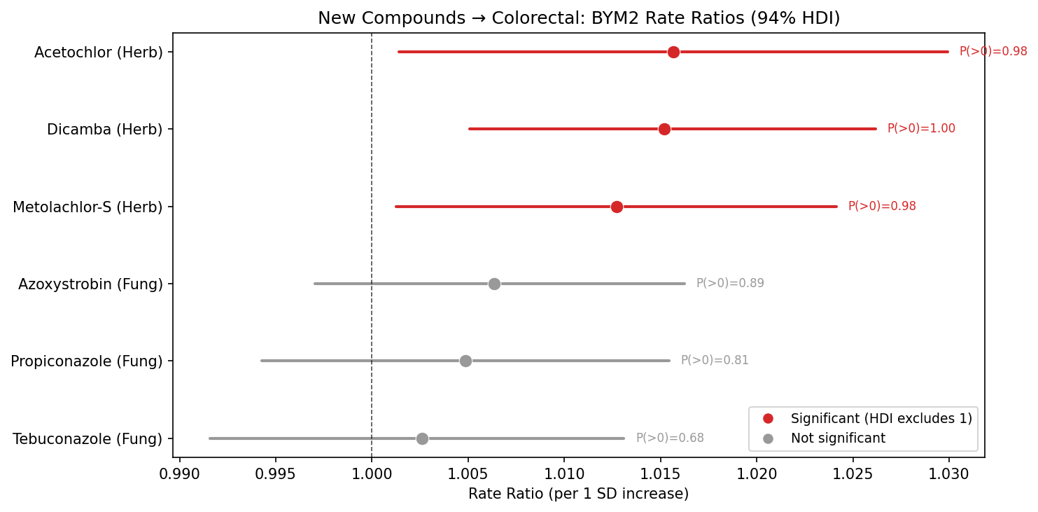
Twelve individual pesticide compounds were tested in separate BYM2 models (each with 12 covariates). The results show clear chemical-class specificity: herbicides are consistently associated with both cancer types, while insecticides are uniformly null.
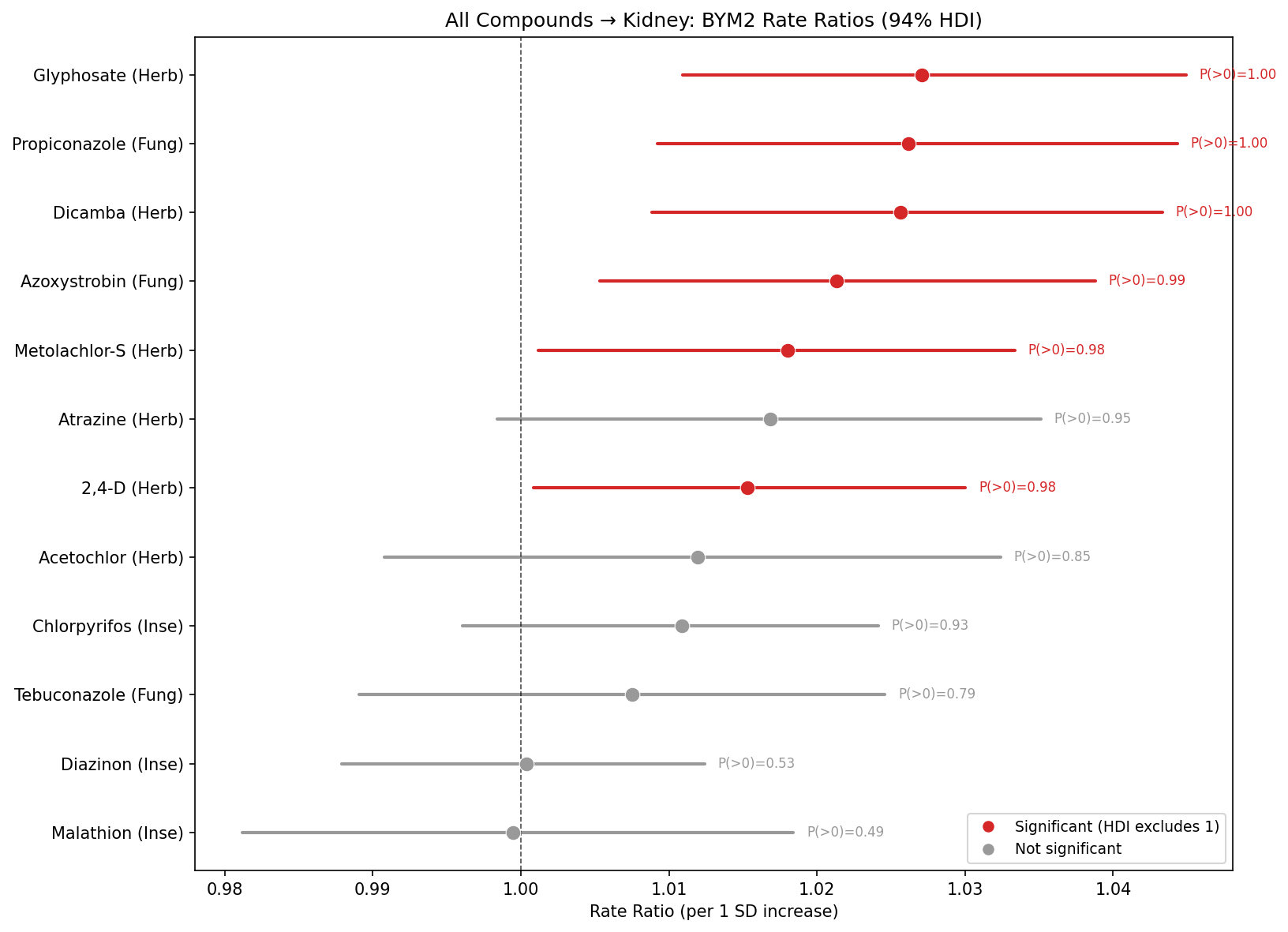
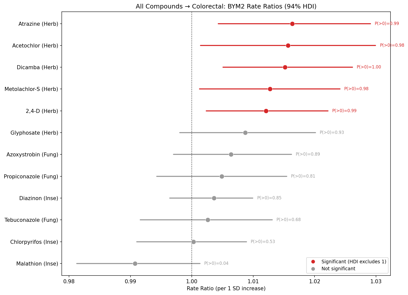
All 12 Compounds: BYM2 Results
| Compound | Class | Cancer | Rate Ratio | 94% HDI | P(>0) | Sig? |
|---|---|---|---|---|---|---|
| Glyphosate | Herbicide | Kidney | 1.027 | [1.011, 1.045] | 0.999 | Yes |
| Glyphosate | Herbicide | Colorectal | 1.009 | [0.998, 1.020] | 0.928 | No |
| Atrazine | Herbicide | Kidney | 1.017 | [0.998, 1.035] | 0.954 | No |
| Atrazine | Herbicide | Colorectal | 1.016 | [1.004, 1.029] | 0.991 | Yes |
| 2,4-D | Herbicide | Kidney | 1.015 | [1.001, 1.030] | 0.977 | Yes |
| 2,4-D | Herbicide | Colorectal | 1.012 | [1.002, 1.022] | 0.988 | Yes |
| Dicamba | Herbicide | Kidney | 1.026 | [1.009, 1.043] | 0.998 | Yes |
| Dicamba | Herbicide | Colorectal | 1.015 | [1.005, 1.026] | 0.997 | Yes |
| Acetochlor | Herbicide | Kidney | 1.012 | [0.991, 1.032] | 0.854 | No |
| Acetochlor | Herbicide | Colorectal | 1.016 | [1.001, 1.030] | 0.981 | Yes |
| Metolachlor-S | Herbicide | Kidney | 1.018 | [1.001, 1.033] | 0.985 | Yes |
| Metolachlor-S | Herbicide | Colorectal | 1.013 | [1.001, 1.024] | 0.983 | Yes |
| Chlorpyrifos | Insecticide | Kidney | 1.011 | [0.996, 1.024] | 0.926 | No |
| Chlorpyrifos | Insecticide | Colorectal | 1.000 | [0.991, 1.009] | 0.525 | No |
| Malathion | Insecticide | Kidney | 0.999 | [0.981, 1.018] | 0.493 | No |
| Malathion | Insecticide | Colorectal | 0.991 | [0.981, 1.001] | 0.038 | No |
| Diazinon | Insecticide | Kidney | 1.000 | [0.988, 1.012] | 0.528 | No |
| Diazinon | Insecticide | Colorectal | 1.004 | [0.996, 1.010] | 0.846 | No |
| Azoxystrobin | Fungicide | Kidney | 1.021 | [1.005, 1.039] | 0.991 | Yes |
| Azoxystrobin | Fungicide | Colorectal | 1.006 | [0.997, 1.016] | 0.891 | No |
| Propiconazole | Fungicide | Kidney | 1.026 | [1.009, 1.044] | 0.997 | Yes |
| Propiconazole | Fungicide | Colorectal | 1.005 | [0.994, 1.015] | 0.811 | No |
| Tebuconazole | Fungicide | Kidney | 1.008 | [0.989, 1.025] | 0.788 | No |
| Tebuconazole | Fungicide | Colorectal | 1.003 | [0.992, 1.013] | 0.677 | No |
Chemical Class Summary
Colorectal cancer shows the cleanest pattern: 5 of 6 herbicides significant, 0 of 3 insecticides, 0 of 3 fungicides. Kidney cancer is muddier—2 fungicides (azoxystrobin, propiconazole) are also significant for kidney, likely reflecting spatial collinearity with herbicide application in agricultural regions.
Causal Identification
Two quasi-causal methods provide evidence beyond cross-sectional association:
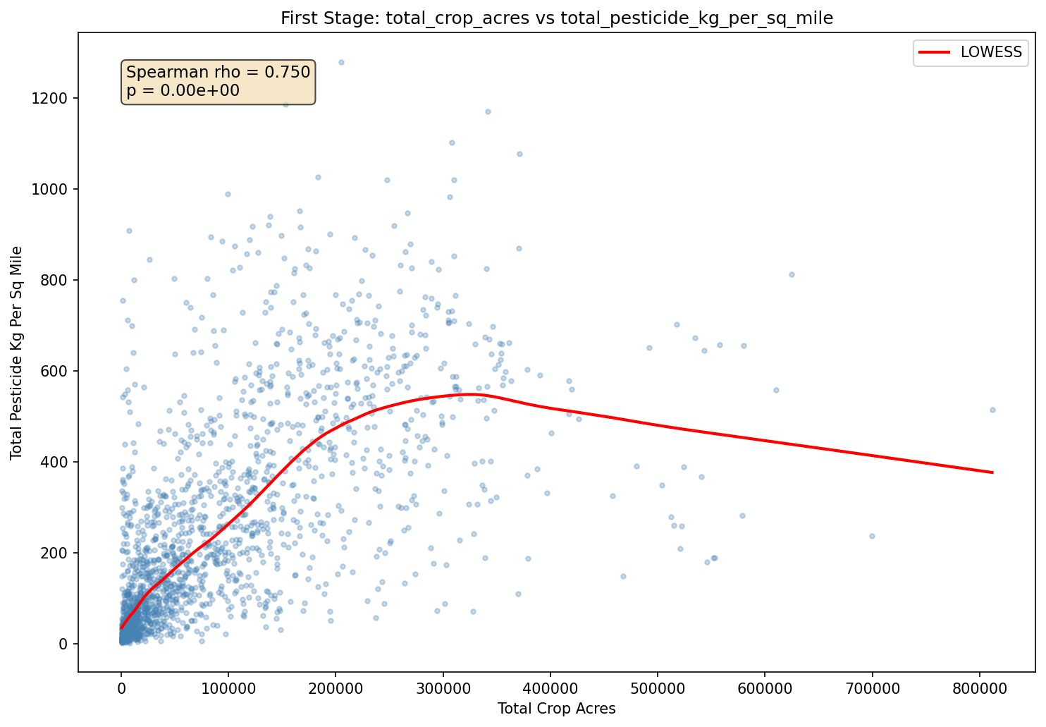
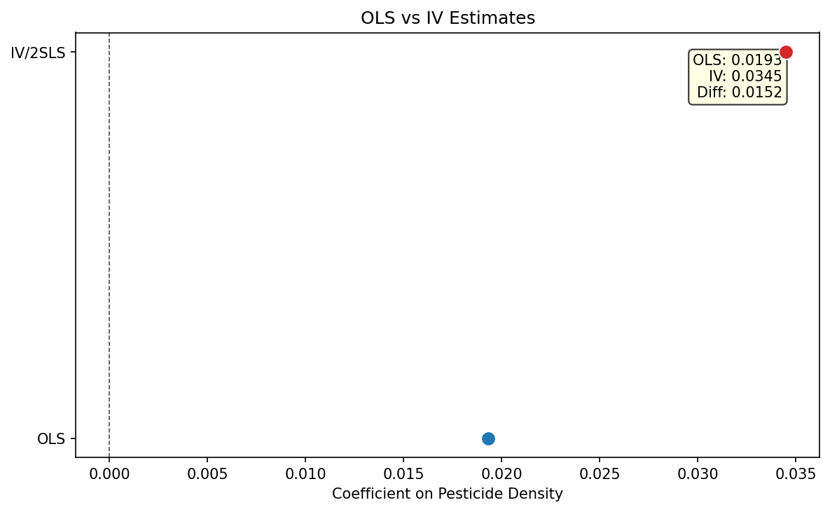
Instrumental Variables (IV/2SLS)
Using total crop acreage as an instrument for pesticide application (first-stage F=377.8, far exceeding the weak-instrument threshold of 10), the IV estimate for pesticide on all-site cancer (0.035) exceeds the OLS estimate (0.019). This pattern—IV > OLS—suggests OLS is attenuated by measurement error in pesticide exposure, not inflated by confounding.
Long-Difference Estimator
Within-county changes in pesticide application from 1997 to 2012 predict changes in cancer incidence. This eliminates all time-invariant confounders (geography, demographics, healthcare access).
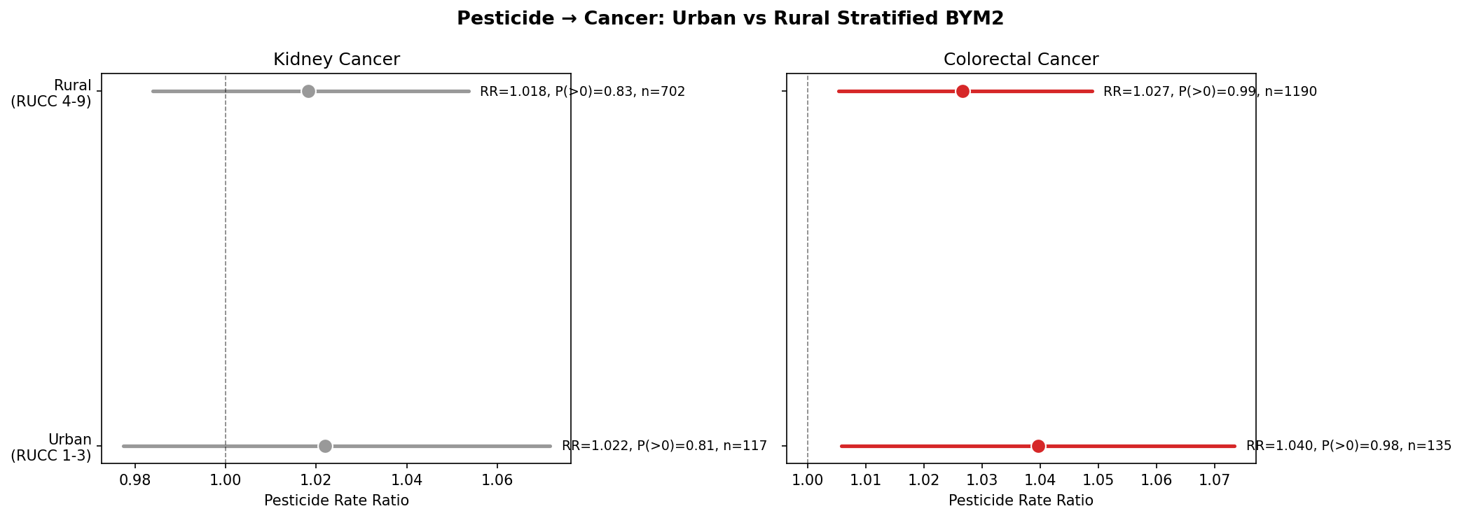
Exposure Pathways
To distinguish occupational from dietary/environmental exposure, BYM2 models were run separately on urban (RUCC 1–3) and rural (RUCC 4–9) counties.
Negative Controls
Several negative control analyses confirm the signal is specific to pesticides and not a proxy for general agricultural intensity or metabolic risk factors:
- Livestock density (hogs, cattle, chickens): 6 of 6 models null for kidney and NHL
- Diabetes prevalence: null for both kidney and colorectal (absorbed by obesity/smoking)
- Fungicides → colorectal: 0 of 3 fungicides significant (herbicides 5/6 significant)
- Insecticides → both cancers: 0 of 6 associations significant
Sensitivity Analyses
Continue Exploring
Risk Factor Gauntlets — See how pesticide associations survive when smoking, obesity, alcohol, and inactivity are modeled as primary exposures.
Exploratory Screening — Hypothesis-free scan of all predictors across 26 cancer types confirms pesticide specificity for kidney and colorectal.
Temporal Trends — Animated maps showing how cancer incidence and pesticide use evolve over time.
Full data tables for all results above are available on the Downloads page. Interactive maps of model outputs are on the Maps page.